~ Introduction
During last year’s OpenZFS Summit I presented the motivation and the internals of the Log Spacemap project - a project that Matt started a long time ago and we ended up finishing together the beginning of this year. In order to fully grasp the context of this post, I highly recommend that you watch last year’s presentation first (link). Regardless, there is still a brief overview in this post, as I believe that the subject discussed can be presented in a more abstract manner.
This post is about the flushing algorithm of the Log Spacemap project that was left as an open question during the aforementioned presentation. It describes the motivation on why an algorithm like that is needed, what were some of the designs that were tried before the one that was implemented, and how does the final design perform. There is also an addendum on the tools that were built around that feature to analyze its behavior.
~ Quick Review of the Log Spacemap feature
Log spacemaps are an optimization in ZFS metadata allocation for pools whose workloads are primarily random-writes (e.g. pools used for databases, VMs, etc..) with high levels of fragmentation. To give some background, each vdev in ZFS is divided into equal parts called metaslabs. ZFS represents each metaslab on-disk with a structure called a spacemap (an append-only log of allocations and frees) and in-memory with an AVL tree where each node represents a range of free space.
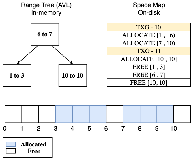
Due to the copy-on-write nature of ZFS, fragmented pools with random-write workloads
end up spending a lot of I/Os each TXG appending to the spacemap of each metaslab.
Instead of doing that, a pool with the Log Spacemap feature enabled logs the
changes of all metaslabs in-memory, in 2 new AVL trees per metaslab (called
unflushed_allocs and unflushed_frees). It also issues a single I/O with all the
metaslab changes in a pool-wide spacemap on-disk (the log spacemap), for persistence.
Persistence is needed specifically for the case that a crash happens and the pool
has to reconstruct its unflushed state (e.g. repopulate unflushed_allocs and
unflushed_frees of each metaslab).
As more blocks are accumulated in log spacemaps and more unflushed changes are accounted in memory, we flush a selected group of metaslabs every TXG for the following reasons:
- Relieve memory pressure
- Decrease overheads in the import time after a crash.
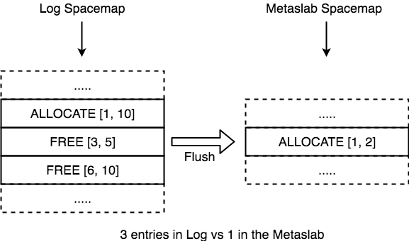
[1] happens as flushing a metaslab means writing all its segments from unflushed_allocs
and unflushed_frees to the metaslab’s spacemap on-disk, after which we can discard
the in-memory unflushed trees. For [2] the situation is a bit more complicated.
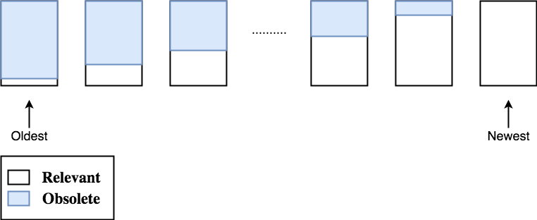
As TXGs pass and we flush metaslabs from oldest-flushed to recently-flushed in a
round-robin fashion, log spacemaps of old TXGs become obsolete. A log spacemap is said
to be obsolete when all its entries have made it to their respective metaslab spacemaps.
Obsolete log spacemaps can be safely destroyed as they are no longer relevant. Obsolete
logs are destroyed every TXG so in the case of an import after a crash we have fewer
log spacemaps to read in order to reconstruct the unflushed state of the pool.
The decision to flush metaslabs in order, from oldest to recently flushed, is essential here as it helps us determine when a log spacemap becomes obsolete. Without having to look at its actual entries, we can be certain that a log spacemap is obsolete if all the metaslabs in the pool have been flushed since the TXG that the spacemap was created. Thus, flushing the oldest-flushed metaslab is always best for helping to delete old log spacemaps.
~ Why is the flushing algorithm important?
There are a few aspects of the Log Spacemap feature that can be problematic if there is no explicit policy on how flushing is handled. The most straightforward one is memory usage. In this new world, each metaslab has 2 extra AVL trees that contain segments which are waiting to be flushed to their metaslab’s spacemap. The more segments are held in memory like this, the bigger the pressure on the system. When we flush a metaslab, we flush all the segments from the aforementioned AVLs to disk, relieving some of this pressure.
The other aspect is the amount of blocks used for log spacemaps on-disk. There should be an explicit limit to keep it in check. If no such limit exists there would be no bound to the overhead induced at import time after a crash. Flushing metaslabs often can help keep the log short. On the other hand, flushing too often defeats the purpose of the log spacemap feature.
To summarize the above, the ideal flushing algorithm should:
- React when the memory usage of the feature is getting out of hand.
- Avoid flushing metaslabs too often in order to minimize the # of I/Os issued.
- Flush metaslabs rarely enough so they utilize their I/O blocksize.
- Flush frequently enough so import times after crashing are not severely impacted.
- Behave in a consistent and predictable manner.
[2] and [3] are antithetical to [4] and this is where reality kicks in. One may say that big enterprise setups of ZFS rarely crash so there is no need to focus on import times after crashing and the goal should be to just make the algorithm rarely flush metaslabs. Regardless of whether this statement is true, crashes do happen. When they do, long import times mean more downtime. Thus, a pragmatic solution to this problem would be to design an algorithm that makes a calculated tradeoff in the amount of flushing that works well enough in the majority of the cases and potentially exposes a knob for expert users that really know what they are doing.
~ Dealing with memory usage
The simplest approach to this is to ensure that the memory usage of the unflushed trees stays below a certain threshold. The threshold can be determined by an arbitrary hard limit (e.g. 1GB is the max amount of memory that can be used by all unflushed changes in the pool), and an arbitrary percentage of the system’s memory (e.g. unflushed changes should not take up more that 0.1% of the system’s memory). From these two, we pick the lowest one as the threshold. Whenever the threshold is exceeded the system starts flushing metaslabs until it gets below it again.
~ Coming up with a block heuristic
Earlier in this post, the use of an explicit limit on the amount of log spacemap blocks was discussed, so the log doesn’t grow indefinitely. For this section we make the simplifying assumption that the block limit is the number of metaslabs on the system. That is not very unreasonable to begin with, as it is discussed in a future section, and it allows us to focus on the flushing algorithm. Before that happens though, it is helpful to define a more abstract model for how log spacemap blocks are deleted on a running system.
The model goes like this: At TXG T, the changes of all the metaslabs in the
pool are written in a log spacemap S and a group of metaslabs G is flushed.
Metaslabs in group G are always chosen in an ordered fashion from oldest-flushed
to recently-flushed from all the metaslabs in the pool. As TXGs pass, more metaslabs
are flushed and entries from S become obsolete. At some point, the system does a
full circle around the metaslabs and has flushed each one of them. At that point it
is guaranteed that all blocks from S are obsolete, and S can be destroyed.
The simplest example of the above model is a hypothetical pool with 10 metaslabs. At TXG 1, we flush metaslab 1 and log all the changes of all metaslabs in log spacemap 1. At TXG 2 we flush metaslab 2, at TXG 3 we flush metaslab 3, ..etc. By TXG 11, we have flushed all the metaslabs once, so we start flushing again from metaslab 1. By that time, even in the worst case that all metaslabs were touched in TXG 1 and all have entries in log 1, all the entries from log 1 are obsolete, because between TXG 1 and 10, we flushed all our metaslabs. Thus we can get rid of log 1 and all of its blocks.
So with the above model in mind we are ready to start coming up with heuristics:
* Block Limit-Only Heuristic
The simplest heuristic would be to just let the limit do the work. In other words, whenever the block limit is exceeded, keep flushing metaslabs until enough blocks are destroyed and the system is again below the limit.
The problem with this approach is visible through the graphs below.
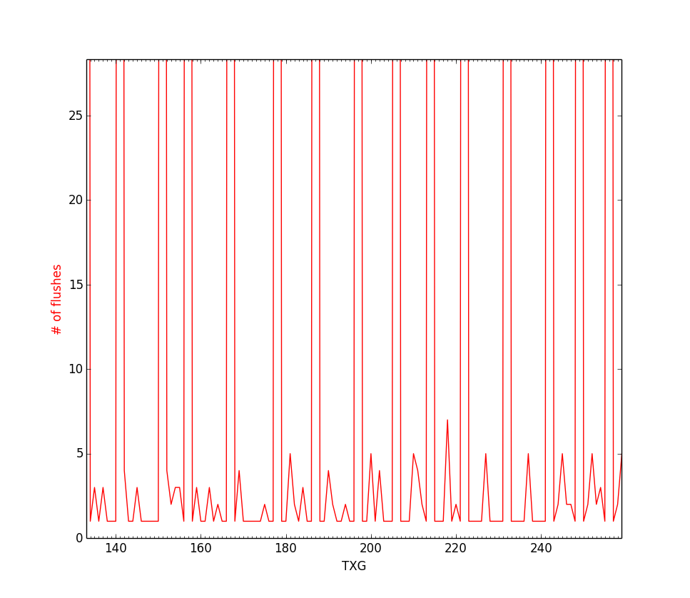
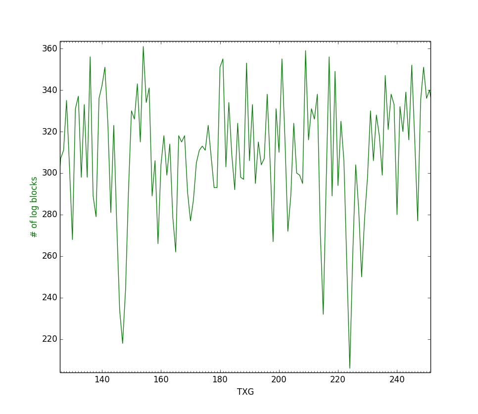
These graphs are part from a larger experiment where we were simulating a pool with ~330 metaslabs (and therefore a block limit of about the same size). The issue here is that no flushing takes place until it is really late, and at that point the majority of the metaslabs are flushed at once. This is far from the ideal. The heuristic is unpredictable and as a result, susceptible to many performance pathologies.
* Average Block and Average Metaslab Heuristic
A better heuristic would take into account the flushing history or the amount of log blocks accumulated so far. Two simple heuristics derived from those ideas are the following:
- Average Metaslabs-Per-Log Heuristic
if block limit is exceeded:
    keep flushing until we go below the limit
else:
    flush X number of metaslabs
        where X is (# of metaslabs) / (# of logs)
The attempt here is to look at the amount of flushing that the system has been doing on average each TXG. Then flush that same amount whenever there is no pressure from the block limit.
- Average Blocks-Per-Log Heuristic
if block limit is exceeded:
    keep flushing until we go below the limit
else:
    flush X number of metaslabs
        where X is (total # of log blocks) / (# of logs)
The idea behind this heuristic is that the system tries to model flushing after the average incoming rate of log blocks per TXG, and thus to flush more when there are many blocks in each log in our history and less when there aren’t many.
Both of the above heuristics are problematic. Average Metaslabs-Per-Log is completely disconnected from the concept of the history of incoming log block rate which can cause problems if the incoming rate is highly variable. On the other hand, Average Blocks-Per-Log is based on this concept but completely misses the concept of the metaslab flushing distribution over the log spacemap history. This makes the heuristic susceptible to the same problems of the Limit-Only heuristic where there are spikes in the flushing behavior because a lot of metaslabs need to be flushed just to destroy a few blocks.
* Running Sums Heuristic
The ideal flushing algorithm takes into consideration the following parameters when deciding how many metaslabs to flush:
- The difference between the total number of log blocks and the block limit.
- The current incoming rate.
- The distribution of metaslabs flushed over the log spacemaps.
- The distribution of log blocks over the log spacemaps.
One design of such an algorithm is the Running Sums heuristic. The main idea behind the heuristic is knowing the answer to the question of “How many metaslabs do we need to flush in order to get rid of X log spacemap blocks?” at any given time. This can be answered by iterating backwards from the oldest log spacemap to the newest one and looking at their metaslab and block counts.
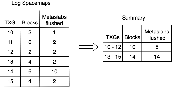
The picture below is an example of the log spacemaps in a pool at some TXG T. For
each log spacemap, we know the number of blocks of the spacemap and the number of
metaslabs flushed at the TXG that it was created. For the oldest log spacemap,
the number of metaslabs flushed in the same TXG that it was created is also the
number of metaslabs that need to be flushed in order for us to destroy it. In the
example below this is 2 metaslabs. For the second oldest log spacemap, the number
of metaslabs that need to be flushed in order for it to get destroyed, is the number
of metaslabs metaslabs needed to destroy the previous log (the oldest one) plus the
number of metaslabs that were flushed in the TXG that it was created. In our example,
that is 5 metaslabs. And so on for the rest of the spacemaps. Doing the same calculations
but in terms of number of log spacemap blocks instead of log spacemaps, the answer
of how many metaslabs we need to flush in order to get rid of 6 log spacemap blocks,
is 2. If we wanted to get rid of 8 or 9 or 10 blocks, then we would need to flush 5
metaslabs.

The more blocks we need to get rid of, the longer the iteration over the log history, over which we basically keep a running sum of the amount of log blocks that we can flush based on the running sum of metaslabs flushed over each log spacemap. This captures the essence of points [3] and [4] of our picture of the ideal flushing algorithm.
With this in mind, the actual behavior of the heuristic works like this: The heuristic projects the incoming rate of the current TXG into the future and attempts to approximate how many metaslabs it needs to flush now in order to avoid exceeding the block limit in different points in the future. These projections are made under the assumption that the incoming rate would stay the same in the future TXGs projected and that the algorithm would be flushing the same number of metaslabs every TXG. Once that is done, the heuristic chooses the maximum number of flushes from all these estimates to be on the safe side. These projections exemplify how points [1] and [2] come into play.
The following picture illustrates an example run of the algorithm.

Running a sample simulation of the algorithm in a hypothetical pool of 300 metaslabs, with incoming blocks chosen randomly between 10 and 64 for a span of 1000 TXGs (same setup as the Block Limit-Only heuristic), we see the following:
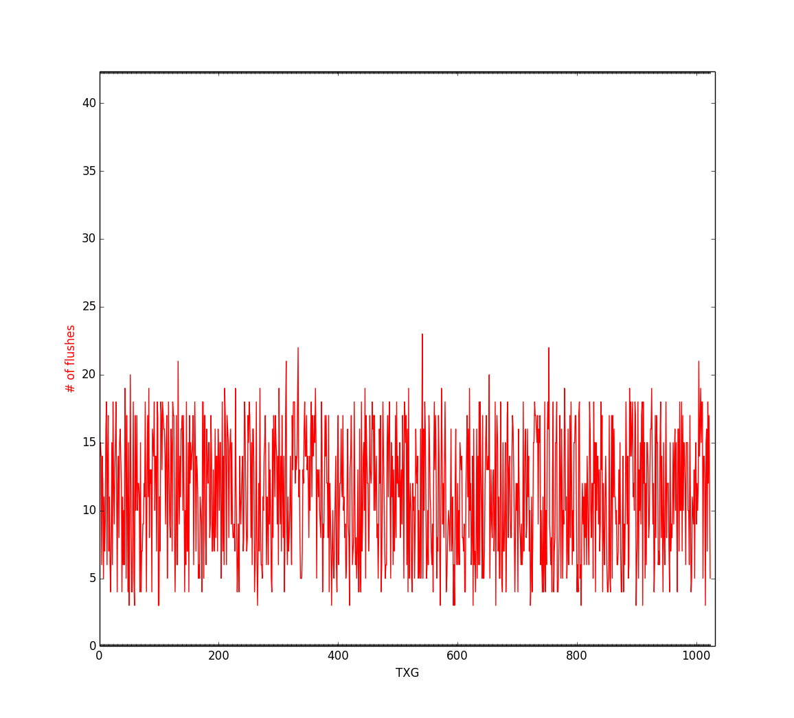
The maximum number of metaslabs ever flushed in a TXG was 24 and the average metaslabs flushed per TXG was 11. That’s close to ~4% of the total number of metaslabs in the pool flushed each TXG on average (with the max being 8%).
~ Towards An Implementation (Running Sums with a Summary)
The above heuristic works great in theory and beats any other heuristic that we’ve come up with in simulations. Unfortunately, there are still some rough edges when it comes to implementing this solution in ZFS. One of them is the assumption that we know the incoming rate of log blocks in the current TXG. This is a bit conflicting in and of itself as we are not able to tell how many log blocks we need to write in the current TXG if the current TXG is not over. Thus, we end up looking at a few (currently 5) TXGs in the past and taking their average as a simple estimation of the incoming rate for the current TXG.
Another important issue is the number of logs that we have to iterate over for this heuristic. The heuristic runs every TXG in syncing context which could potentially induce a lot of overhead in the system’s runtime. For this reason, we always maintain a summary table of log blocks and metaslab counts between TXGs and iterate over that, instead of the actual log spacemaps. The tradeoff here is basically giving up some accuracy on our flushing estimates for a decrease in the runtime of the heuristic. That said, trying out the algorithm with and without a summary in a simulation yield very similar results in flushing behavior. Below you can see the summary of the log history from the previous section.
All of the above heuristics and their behavior were compared in simulations run in the following simulator:
Feel free to give it a run. Unfortunately this was a side-project, so the project’s documentation didn’t get the love it deserved. That said, reading the code should be straightforward.
~ Reconsidering the hard limit for our block heuristic
The Running Sums heuristic makes the decision of the hard limit of log blocks more critical than before, as the heuristic itself adapts its flushing behavior based on the distance between the current number of log blocks and the limit.
In other words, the value of the limit affects the flushing algorithm, with higher values flushing metaslabs less often (doing less I/Os) per TXG and lower values flushing metaslabs more aggressively with the upside of saving overheads when loading the pool after a crash. Another factor in this tradeoff is that flushing less often can potentially lead to better utilization of the metaslab spacemap’s block size as we accumulate more changes per flush.
Given that the limit indirectly controls the flush rate (metaslabs flushed per TXG) we decided to implement it as a tunable expressed as a percentage in terms of the number of metaslabs in the pool. As for setting a default, the idea is the following: If the whole log were to be flushed, each metaslab would be flushed once. To make the most of each flush, we would want to write at least one whole block to each metaslab’s spacemap. Thus, we want the amount of data in all the log spacemaps to to be at least equal to the number of metaslabs, in terms of metaslab spacemap blocks, when flushed.
With that in mind, we decided to make this tunable to be 4 times the number of metaslabs in the pool with the following assumptions in mind:
- Assuming a constant flush rate and a constant incoming rate of log blocks it is reasonable to expect that the amount of obsolete entries changes linearly from TXG to TXG (e.g. the oldest log should have the most obsolete entries, and the most recent one the least). With this we can say that, at any given time, about half of the entries in the whole spacemap log are obsolete. Thus, for every two entries for a metaslab in the log space map, only one of them is valid and actually makes it to the metaslab’s space map. That gives us a factor of 2.
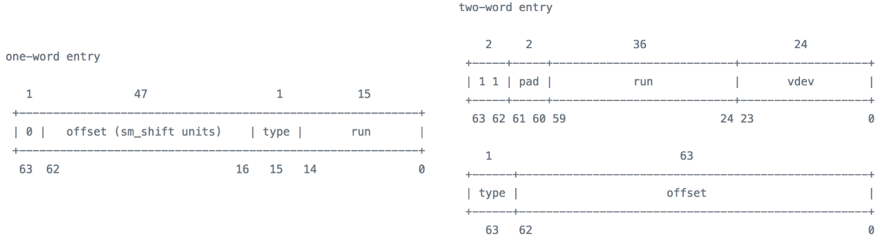
- Each entry in the log spacemap is guaranteed to be two words while entries in metaslab spacemaps are generally single-word. Which gives us another factor of 2.
- Even if [1] and [2] are slightly less than a factor of 2 each in reality, we haven’t taken into account any consolidation of segments from the log spacemap to the unflushed range trees nor their history (e.g. a segment being allocated, then freed, then allocated again means 3 log spacemap entries but 0 metaslab space map entries).
The above assumptions are workload dependent. For example, we’ve seen a factor of ~1.8 non-obsolete log space map entries per metaslab entry, which could make the case to set the default of the tunable to be 6 times the number of metaslabs. Again, taking the conservative approach we kept that factor to 4.
~ “Limiting” the value of the block limit
In large pools with many metaslabs the limit of the block heuristic can easily get out of hand which could make import times after crashes painful. Thus, regardless of the number of metaslabs in a system there needs to be an upper bound to the block limit and therefore to the import time overhead. At the same time, the bound should be set with caution because if it is too low it could penalize performance on SSDs (the idea being that SSDs can have a significantly higher incoming rate of log blocks and thus flush more often than HDDs under the same block limit).
Assuming that 1TB SSDs become the standard (if they are not already?) a pool with such a drive should have ~64K metaslabs, thus according to our scheme of factor of 4, the block limit should be 256K log blocks.
Now assuming a steady incoming rate of ~200 log blocks per TXG on such an SSD, then the pool should be flushing:
(log blocks per TXG / [(log block size) / (metaslab spacemap size)] / block limit factor)
or
200 / 2 / 4 = 25
25 metaslabs per TXG in order to stay under the limit. Thus, if we were to
hypothetically get rid of the whole spacemap log with that flushing rate it would
take 2560 TXGs [= 64K metaslabs / 25 metaslabs flushed per TXG] (this is
basically how many TXGs it would take us to flush all the metaslabs in the pool).
In a span of that many TXGs and the steady incoming rate stated above, the
cumulative size of all our log spacemaps should be
[2560 TXGs * 200 log blocks per TXG =] 512K log blocks.
This means that if the log block limit is less than 512K, the system will flush more than 1 metaslab per log block. We decided to default the limit to half of that (256K), as import times would take a huge hit for HDDs at this point. This makes the above SSD scenario flush 2 metaslabs per log block (or 1 metaslab per half log block if you prefer), which should theoretically still be fine for an SSD.
Finally, there is a need for a lower bound in the block limit for lower-end systems with small pools and a small number of metaslabs. The problem here is that if the number of metaslabs is small and the incoming rate is high, the system may end up flushing all the metaslabs every TXG. Thus, we don’t allow the limit be less than 1000 log blocks. (The number was decided based on a theoretical pool with a single small vdev that can reach 100 IOPS and its target import time is 10 seconds at worst).
~ Performance Results
Below are the graphs displaying the performance improvements of this optimization from a 5-day experiment. The experiment involved 2 pools whose workloads were random-writes, with one of them having the feature enabled. We left the experiment to run long enough so both of the pools would reach a steady state and high levels of fragmentation (both pools reached 91~92% fragmentation at their steady states). The graphs display the userland IOPS reached by the pool per second. This is the most practical metric for such an experiment as more userland IOPS means more work done for your applications.
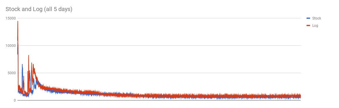
The above graph verifies that the pools had reached their steady state (no fluctuations on IOPS). The graph below emphasizes the last 10 hours of the experiment:
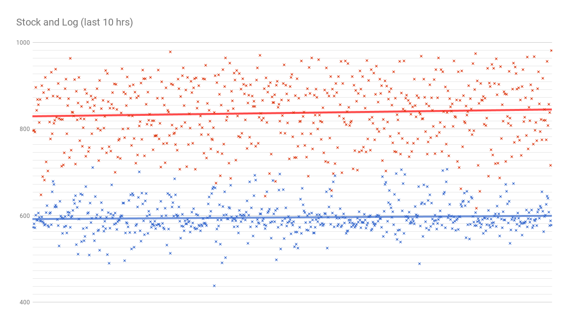
For those last 10 hours the average IOPS for the stock bits were ~596 IOPS. On the other hand, the pool with the log spacemap enabled had an average of ~837 IOPS. For this experiment the log spacemap optimization gave a ~40.5% improvement over the stock bits on a steady state under high fragmentation.
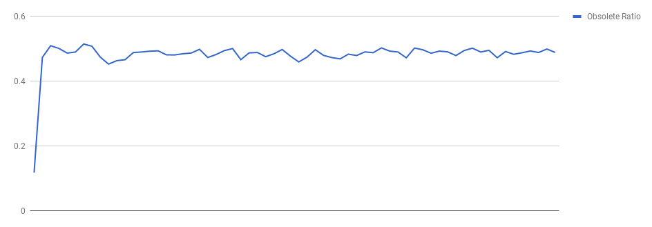
~ Verifying our assumptions
Earlier while considering the limit to our block heuristic we made the assumption that half of the entries in the log are obsolete. For completeness, the graphs below verify this hypothesis under our experiment:
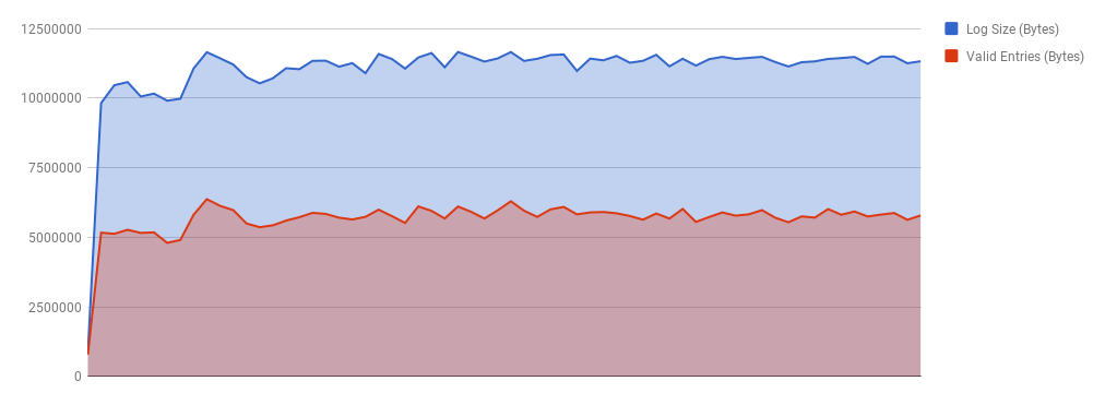
As for consolidation (how many log spacemap segments do we have per metaslab spacemap segments), we found the ratio to be ~1.87, after sampling a few metaslabs.
~ Analysis on a running system
Even though we tried our best to provide good defaults for this feature and avoid any performance pathologies that we could think of, we can’t really foresee every workload that a pool with this feature enabled will experience. As a result, we made sure to implement a lot of introspection in the behavior of the feature.
zdb can now print:
- the TXG where each metaslab was last flushed
$ sudo zdb rpool
...
        metaslab      1   offset     20000000   spacemap     58   free     496M
        On-disk histogram:              fragmentation 7
                          9:      8 *******
                         10:      6 *****
                         11:      4 ****
                         12:      3 ***
                         13:      4 ****
                         14:      8 *******
                         15:     38 ******************************
                         16:     28 **********************
                         17:     51 ****************************************
                         18:     34 ***************************
                         19:     28 **********************
                         20:     23 *******************
                         21:     18 ***************
                         22:      5 ****
                         23:      5 ****
                         24:      6 *****
                         25:      1 *
                         26:      1 *
space map object 58:
  smp_length = 0x2d1b0
  smp_alloc = 0x1016800
        Flush data:
        unflushed txg=23350   # <----- HERE
...
- the contents of each log spacemap
$ sudo zdb -mmmm rpool
...
Log Space Maps in Pool:
Log Spacemap object 23569 txg 23357
space map object 23569:
  smp_length = 0x13a8
  smp_alloc = 0xfffffffffff30200
            [     0] ALLOC: txg 23357 pass 1
            [     1]    A  range: 0187f53e00-0187f55e00  size: 002000 vdev: 000000 words: 2
            [     2]    A  range: 0195d49e00-0195d4be00  size: 002000 vdev: 000000 words: 2
            [     3] FREE: txg 23357 pass 1
            [     4]    F  range: 0187cd5e00-0187cd7e00  size: 002000 vdev: 000000 words: 2
            [     5]    F  range: 0195d43c00-0195d44400  size: 000800 vdev: 000000 words: 2
            [     6]    F  range: 0195d44600-0195d45800  size: 001200 vdev: 000000 words: 2
            [     7]    F  range: 0195d4aa00-0195d4ac00  size: 000200 vdev: 000000 words: 2
            [     8] ALLOC: txg 23357 pass 1
            [     9]    A  range: 010fccfc00-010fcd6400  size: 006800 vdev: 000000 words: 2
            [    10]    A  range: 0116f94a00-0116fd3600  size: 03ec00 vdev: 000000 words: 2
            [    11] FREE: txg 23357 pass 1
            [    12]    F  range: 0100000000-0100010000  size: 010000 vdev: 000000 words: 2
            [    13]    F  range: 010fc18c00-010fc21400  size: 008800 vdev: 000000 words: 2
            [    14]    F  range: 010fc22400-010fc31400  size: 00f000 vdev: 000000 words: 2
            [    15]    F  range: 010fc37c00-010fc46c00  size: 00f000 vdev: 000000 words: 2
            [    16]    F  range: 0114a32600-0114a44600  size: 012000 vdev: 000000 words: 2
...
- the amount of valid (non-obsolete) entries for each log spacemap
$ sudo zdb -vvvv rpool
Log Space Map Obsolete Entry Statistics:
0        valid entries out of 115      - txg 23315
0        valid entries out of 110      - txg 23316
0        valid entries out of 182      - txg 23317
0        valid entries out of 172      - txg 23318
22       valid entries out of 210      - txg 23319
13       valid entries out of 121      - txg 23320
13       valid entries out of 107      - txg 23321
12       valid entries out of 112      - txg 23322
24       valid entries out of 170      - txg 23323
30       valid entries out of 160      - txg 23324
30       valid entries out of 151      - txg 23325
35       valid entries out of 232      - txg 23326
15       valid entries out of 115      - txg 23327
26       valid entries out of 101      - txg 23328
43       valid entries out of 158      - txg 23329
48       valid entries out of 210      - txg 23330
23       valid entries out of 99       - txg 23331
26       valid entries out of 110      - txg 23332
46       valid entries out of 114      - txg 23333
55       valid entries out of 124      - txg 23334
67       valid entries out of 154      - txg 23335
134      valid entries out of 242      - txg 23336
...
Some known mdb dcmds were extended and new ones where introduced:
::spa -mand::vdev -Mhave a new column called UCMU (stands for Unflushed Changes Memory Usage).
> ::spa -m
ADDR                 STATE NAME
ffffff1975b30000    ACTIVE apollo

    ADDR             STATE     AUX          DESCRIPTION
    ffffff19689be000 HEALTHY   -            root
    ffffff1960e51000 HEALTHY   -              /dev/dsk/c2t4d0s0
        ADDR                 ID               OFFSET       FREE       FRAG       UCMU
        ffffff1c3598fb40      0                    0       480M        79%      98.6K
        ffffff1a01aa4040      1             20000000       445M        80%       115K
        ffffff19b3e78980      2             40000000       431M        79%      69.0K
        ffffff1c35d1fb80      3             60000000       441M        72%       119K
        ffffff1c35a4b6c0      4             80000000       420M        82%       101K
        ....
> ffffff038429e000::vdev -M
ADDR             STATE     AUX          DESCRIPTION
ffffff038429e000 HEALTHY   -            /dev/dsk/c2t1d0s0
    ADDR                FRAG      UCMU
    ffffff03da3b5000      0%       256
    ...
::spa_spacealso includes unflushed changes
> ffffff1975b30000::spa_space
dd_space_towrite = 0M 10865M 7926M 0M
dd_phys.dd_used_bytes = 53505M
dd_phys.dd_compressed_bytes = 53202M
dd_phys.dd_uncompressed_bytes = 154736M
ms_allocmap = 0M 717M 0M 0M
ms_checkpointing = 0M
ms_freeing = 707M
ms_freed = 0M
ms_unflushed_frees = 4665M
ms_unflushed_allocs = 5175M
ms_allocatable = 14454M
ms_deferspace = 2173M
current avail = 150270M
::logsm_statsprints the table and summary of the block heuristic
> ::walk spa |::logsm_stats
Log Entries:
txg     blks    ms      obj
8235    10      7       8679
8236    11      8       8680
8237    10      9       8681
8238    10      3       8682
...

Summary Entries:
start-txg       blks    ms
8232            10      7
8236            41      22
8240            40      12
...
Experimental kstats were also added. Once stabilized these metrics can be used by monitoring tools.
$ kstat -m zfs -c pool
module: zfs                             instance: 0
name:   0x22557e79f5e7be7b              class:    pool
        crtime                          35.210331320
        metadata_blocks                 29900
        metaslab_flushes                29992
        pool_name                       rpool
        snaptime                        1494585.398219727
        txgs                            30697
And of course a DTrace script (see addendum).
~ Acknowledgements
I am grateful to Matt Ahrens and the management at Delphix that gave me the opportunity to work on this project, my team for their feedback and support, and the following people that went the extra mile in helping me edit all of my material and present it: John Gallagher, Sara Hartse, Amanda Merriweather, and my sisters Dina and Margarita.
~ Addendum:
Log Spacemap Flushing Stats:
$ cat ~/scripts/logsm_stats.xd
#!/usr/sbin/dtrace -Cqs

spa_t *spa;
uint64_t log_sm_blksz;

uint64_t txg;
uint64_t nblocks_added;
uint64_t total_nblocks;
uint64_t total_nlogs;
uint64_t metaslabs_flushed;

spa_sync:entry
/!spa && stringof(args[0]->spa_name) == $$1/
{
	spa = args[0];
	log_sm_blksz = (1 << 17); /* 128K */
}

spa_sync:entry
/spa && args[0] == spa/
{
	txg = args[1];
}

metaslab_flush_update:entry
/spa && args[0]->ms_group->mg_vd->vdev_spa == spa/
{
	metaslabs_flushed++;
}

space_map_close:entry
/spa && args[0] == spa->spa_syncing_log_sm/
{
	total_nlogs = spa->spa_sm_logs_by_txg.avl_numnodes;
	nblocks_added =
	    spa->spa_syncing_log_sm->sm_phys->smp_length / log_sm_blksz;

	rem = spa->spa_syncing_log_sm->sm_phys->smp_length % log_sm_blksz;
	if (rem != 0) {
		nblocks_added += 1;
	}
}

spa_sync:return
/spa && entry->args[0] == spa/
{
	total_nblocks = spa->spa_unflushed_stats.sus_nblocks;

	printf("txg %u | %u +blocks | %u total_blocks | %u logs | %u flushed | %Y\n",
	    txg, nblocks_added, total_nblocks, total_nlogs, metaslabs_flushed, walltimestamp);

	txg               = 0;
	nblocks_added     = 0;
	total_nblocks     = 0;
	total_nlogs       = 0;
	metaslabs_flushed = 0;
}

$ sudo logsm_stats.xd
txg 11176 | 13 +blocks | 1462 total_blocks | 108 logs | 21 flushed | 2018 Feb  5 15:35:03
txg 11177 | 12 +blocks | 1460 total_blocks | 108 logs | 18 flushed | 2018 Feb  5 15:35:19
txg 11178 | 13 +blocks | 1457 total_blocks | 108 logs | 16 flushed | 2018 Feb  5 15:35:43
txg 11179 | 13 +blocks | 1445 total_blocks | 107 logs | 19 flushed | 2018 Feb  5 15:36:08
txg 11180 | 15 +blocks | 1448 total_blocks | 107 logs | 16 flushed | 2018 Feb  5 15:36:35
txg 11181 | 13 +blocks | 1446 total_blocks | 107 logs | 19 flushed | 2018 Feb  5 15:36:57
txg 11182 | 14 +blocks | 1430 total_blocks | 106 logs | 17 flushed | 2018 Feb  5 15:37:24
txg 11183 | 16 +blocks | 1446 total_blocks | 107 logs | 8 flushed | 2018 Feb  5 15:38:00
txg 11184 | 16 +blocks | 1449 total_blocks | 107 logs | 20 flushed | 2018 Feb  5 15:38:29
txg 11185 | 16 +blocks | 1465 total_blocks | 108 logs | 4 flushed | 2018 Feb  5 15:39:02
...